Here is a Python program to perform Exploratory Data Analysis (EDA) on the Titanic dataset. It includes steps like loading the data, checking for missing values, visualizing distributions, and analyzing correlations.

# Importing Libraries
import pandas as pd
import numpy as np
import seaborn as sns
import matplotlib.pyplot as plt

# Load the Titanic dataset
# Replace 'your_dataset.csv' with your actual Titanic dataset file path
df = pd.read_csv('your_dataset.csv')

# Set up visualizations style
sns.set(style="whitegrid")
plt.rcParams["figure.figsize"] = (10, 6)

# Display basic information about the dataset
print("Dataset Information:")
print(df.info())

print("\nSummary Statistics:")
print(df.describe())

# Check for missing values
print("\nMissing Values:")
print(df.isnull().sum())

# Handle missing values for EDA (filling or dropping)
df['Age'].fillna(df['Age'].median(), inplace=True)
df['Embarked'].fillna(df['Embarked'].mode()[0], inplace=True)

# Univariate Analysis
# 1. Distribution of 'Survived'
sns.countplot(x='Survived', data=df, palette='pastel')
plt.title('Survival Count')
plt.show()

# 2. Gender distribution
sns.countplot(x='Sex', data=df, palette='pastel')
plt.title('Gender Count')
plt.show()

# 3. Passenger Class distribution
sns.countplot(x='Pclass', data=df, palette='pastel')
plt.title('Passenger Class Distribution')
plt.show()

# 4. Distribution of Age
sns.histplot(df['Age'], kde=True, bins=30, color='blue')
plt.title('Age Distribution')
plt.show()

# Bivariate Analysis
# 1. Survival by Gender
sns.countplot(x='Sex', hue='Survived', data=df, palette='pastel')
plt.title('Survival by Gender')
plt.show()

# 2. Survival by Passenger Class
sns.countplot(x='Pclass', hue='Survived', data=df, palette='pastel')
plt.title('Survival by Passenger Class')
plt.show()

# 3. Survival by Embarkation Port
sns.countplot(x='Embarked', hue='Survived', data=df, palette='pastel')
plt.title('Survival by Embarkation Port')
plt.show()

# Correlation Analysis
# Encode categorical variables for correlation analysis
df_encoded = df.copy()
df_encoded['Sex'] = df_encoded['Sex'].map({'male': 0, 'female': 1})
df_encoded['Embarked'] = df_encoded['Embarked'].map({'C': 0, 'Q': 1, 'S': 2})

# Heatmap of correlations
corr_matrix = df_encoded.corr()
sns.heatmap(corr_matrix, annot=True, cmap='coolwarm')
plt.title('Correlation Matrix')
plt.show()

# Additional Insights
# 1. Survival by Fare
sns.boxplot(x='Survived', y='Fare', data=df, palette='pastel')
plt.title('Fare vs Survival')
plt.show()

# 2. Age vs Survival
sns.boxplot(x='Survived', y='Age', data=df, palette='pastel')
plt.title('Age vs Survival')
plt.show()

# 3. SibSp and Parch Analysis
sns.countplot(x='SibSp', hue='Survived', data=df, palette='pastel')
plt.title('Survival by Number of Siblings/Spouses')
plt.show()

sns.countplot(x='Parch', hue='Survived', data=df, palette='pastel')
plt.title('Survival by Number of Parents/Children')
plt.show()

print("EDA Completed!")

Steps in the Program:

1. Loading the Dataset:
   • Loads the Titanic dataset using pandas.
2. Data Overview:
   • Prints dataset structure, summary statistics, and checks for missing values.
3. Handling Missing Values:
   • Fills missing values in Age with the median and Embarked with the mode.
4. Univariate Analysis:
   • Visualizes the distribution of key variables (Survived, Sex, Pclass, Age).
5. Bivariate Analysis:
   • Examines relationships between survival and variables like Sex, Pclass, Embarked, Fare, and Age.
6. Correlation Analysis:
   • Converts categorical variables to numeric for correlation analysis and visualizes the correlation matrix.
7. Insights from SibSp and Parch:
   • Analyzes the effect of family size on survival.

Output:

This program will generate several plots, such as:

• Count plots for survival and other categorical variables.
• Histograms and boxplots for numerical variables.
• Heatmap for correlations.

You can expand this code further based on specific EDA requirements.

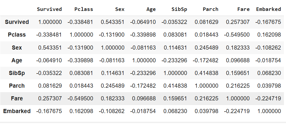
What is Correlation Matrix

The correlation matrix provided shows how strongly each variable is linearly associated with the target variable Survived in the Titanic dataset. Correlation values range from -1 to 1:

• Positive Correlation: Indicates that as the feature increases, the likelihood of survival increases (closer to +1).
• Negative Correlation: Indicates that as the feature increases, the likelihood of survival decreases (closer to -1).
• Close to 0: Indicates little to no linear relationship with survival.

Breakdown of Correlations:

1. Survived with Pclass (-0.338481):
   • Negative correlation: Passengers in higher classes (lower numerical value, e.g., 1 for 1st class) had a better chance of survival. Conversely, those in lower classes (e.g., 3rd class) had a reduced chance of survival.
2. Survived with Sex (0.543351):
   • Strong positive correlation: Being female significantly increased the likelihood of survival. This aligns with the historical context of “women and children first” during the Titanic disaster.
3. Survived with Age (-0.06491):
   • Weak negative correlation: Older passengers had a slightly lower likelihood of survival, though the relationship is weak and may not be significant.
4. Survived with SibSp (-0.035322):
   • Very weak negative correlation: The number of siblings or spouses a passenger had onboard has little to no relationship with survival.
5. Survived with Parch (0.081629):
   • Weak positive correlation: Passengers traveling with parents or children had a slightly better chance of survival, though the relationship is not strong.
6. Survived with Fare (0.257307):
   • Moderate positive correlation: Passengers who paid higher fares had a better chance of survival. This could be because higher fares often corresponded to higher-class tickets (1st class), which had better access to lifeboats.
7. Survived with Embarked (-0.167675):
   • Negative correlation: The port of embarkation is weakly related to survival. For example, passengers embarking from certain ports (e.g., Southampton) might have been more likely to be in lower classes, indirectly affecting survival rates.

Insights:

• Strongest Predictor: Sex (0.543351) is the most significant factor, highlighting that females had a better chance of survival.
• Class Matters: Both Pclass (-0.338481) and Fare (0.257307) show that socioeconomic status (1st class vs. 3rd class) influenced survival rates.
• Weak Predictors: Age, SibSp, and Parch have weak correlations, meaning their impact on survival is minimal compared to other variables.
• Embarked: Though weakly correlated, this variable may reflect indirect effects like the class of travel, which ties to survival.

Recommendations:

While correlation gives a linear perspective, decision trees or other models can capture non-linear relationships. Features like Pclass, Sex, and Fare should be prioritized in predictive modeling due to their stronger correlations with survival.