In Power BI we already did Exploratory data analysis and you can find the tutorials here

Quick overview of the steps

1. Load data (CSV)
2. Quick EDA and cleaning
3. Feature engineering & encoding
4. Train/test split and scale (where needed)
5. Baseline model (Linear Regression)
6. Stronger models: Random Forest & XGBoost + cross-validation
7. Hyperparameter tuning (RandomizedSearchCV)
8. Evaluate with MAE / RMSE / R²
9. Save the best model
10. Example: predict on new row

# 0. Install dependencies (if not already installed)
# !pip install pandas numpy scikit-learn xgboost joblib seaborn matplotlib

import pandas as pd
import numpy as np
import seaborn as sns
import matplotlib.pyplot as plt

from sklearn.model_selection import train_test_split, cross_val_score, RandomizedSearchCV
from sklearn.preprocessing import StandardScaler, OneHotEncoder
from sklearn.compose import ColumnTransformer
from sklearn.pipeline import Pipeline
from sklearn.metrics import mean_absolute_error, mean_squared_error, r2_score
from sklearn.linear_model import Ridge
from sklearn.ensemble import RandomForestRegressor
import xgboost as xgb
import joblib
import warnings
warnings.filterwarnings("ignore")

# -------------------------
# 1) Load dataset
# -------------------------
# NOTE: replace file_url with your actual CSV path if needed.
file_url = "data/housing.csv"  # <-- replace with actual CSV path like "/mnt/data/housing.csv"
# If the file is an image (the path above), replace it with the CSV path before running.
# Example: file_url = "/data/housing.csv"

df = pd.read_csv(file_url)
print("Loaded dataset shape:", df.shape)
display(df.head())

# -------------------------
# 2) Quick EDA & cleaning
# -------------------------
print("\nData types:\n", df.dtypes)
print("\nMissing values:\n", df.isna().sum())

# Basic statistics
display(df.describe())

# Convert typical yes/no to binary if present (some columns contain 'yes'/'no')
binary_cols = ['mainroad', 'guestroom', 'basement', 'hotwaterheating', 'airconditioning', 'prefarea']
for c in binary_cols:
    if c in df.columns:
        df[c] = df[c].map({'yes':1, 'no':0}).astype(int)

# If furnishingstatus is categorical with values like 'furnished','semi_furnished','unfurnished'
if 'furnishingstatus' in df.columns:
    df['furnishingstatus'] = df['furnishingstatus'].astype(str)

# Remove or cap obvious outliers if needed (example: price or area)
# Example: remove rows where price <= 0
df = df[df['price'] > 0].copy()

# -------------------------
# 3) Feature engineering
# -------------------------
# Create useful features: price per sqft, maybe interaction terms
if 'price' in df.columns and 'area' in df.columns:
    df['price_per_sqft'] = df['price'] / (df['area'].replace({0:np.nan}))
    df['price_per_sqft'] = df['price_per_sqft'].fillna(df['price_per_sqft'].median())

# Example: total_rooms could be bedrooms + bathrooms
if 'bedrooms' in df.columns and 'bathrooms' in df.columns:
    df['total_rooms'] = df['bedrooms'] + df['bathrooms']

# Drop columns that are identifiers (none in provided dataset), e.g. 'id'
# df = df.drop(columns=['id'], errors='ignore')

# -------------------------
# 4) Prepare features and target
# -------------------------
TARGET = 'price'
X = df.drop(columns=[TARGET])
y = df[TARGET].values

# Identify numeric and categorical columns
numeric_cols = X.select_dtypes(include=['int64','float64']).columns.tolist()
cat_cols = X.select_dtypes(include=['object','category']).columns.tolist()

print("Numeric columns:", numeric_cols)
print("Categorical columns:", cat_cols)

# -------------------------
# 5) Train / Test split
# -------------------------
X_train, X_test, y_train, y_test = train_test_split(X, y, test_size=0.2, random_state=42)
print("Train shape:", X_train.shape, "Test shape:", X_test.shape)

# -------------------------
# 6) Preprocessing pipelines
# -------------------------
# Numeric pipeline: scale
numeric_transformer = Pipeline(steps=[
    ('scaler', StandardScaler())
])

# Categorical pipeline: OneHot
categorical_transformer = Pipeline(steps=[
    ('onehot', OneHotEncoder(handle_unknown='ignore', sparse=False))
])

preprocessor = ColumnTransformer(transformers=[
    ('num', numeric_transformer, numeric_cols),
    ('cat', categorical_transformer, cat_cols)
], remainder='drop')

# -------------------------
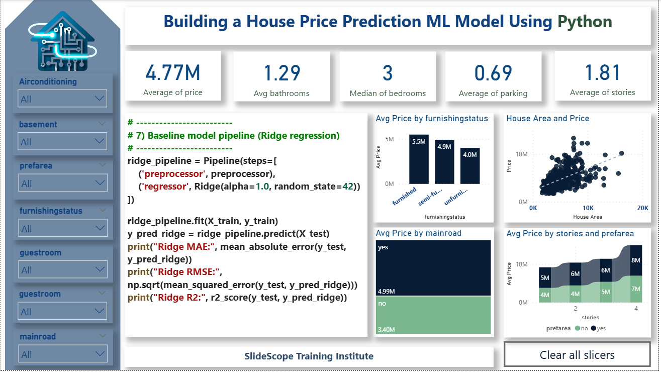
# 7) Baseline model pipeline (Ridge regression)
# -------------------------
ridge_pipeline = Pipeline(steps=[
    ('preprocessor', preprocessor),
    ('regressor', Ridge(alpha=1.0, random_state=42))
])

ridge_pipeline.fit(X_train, y_train)
y_pred_ridge = ridge_pipeline.predict(X_test)
print("Ridge MAE:", mean_absolute_error(y_test, y_pred_ridge))
print("Ridge RMSE:", np.sqrt(mean_squared_error(y_test, y_pred_ridge)))
print("Ridge R2:", r2_score(y_test, y_pred_ridge))

# -------------------------
# 8) Random Forest (stronger baseline)
# -------------------------
rf_pipeline = Pipeline(steps=[
    ('preprocessor', preprocessor),
    ('regressor', RandomForestRegressor(n_estimators=200, max_depth=12, n_jobs=-1, random_state=42))
])
rf_pipeline.fit(X_train, y_train)
y_pred_rf = rf_pipeline.predict(X_test)
print("\nRandom Forest MAE:", mean_absolute_error(y_test, y_pred_rf))
print("Random Forest RMSE:", np.sqrt(mean_squared_error(y_test, y_pred_rf)))
print("Random Forest R2:", r2_score(y_test, y_pred_rf))

# -------------------------
# 9) XGBoost (often best for tabular)
# -------------------------
xgb_pipeline = Pipeline(steps=[
    ('preprocessor', preprocessor),
    ('regressor', xgb.XGBRegressor(n_estimators=300, learning_rate=0.05, max_depth=6, n_jobs=-1, random_state=42))
])
xgb_pipeline.fit(X_train, y_train)
y_pred_xgb = xgb_pipeline.predict(X_test)
print("\nXGBoost MAE:", mean_absolute_error(y_test, y_pred_xgb))
print("XGBoost RMSE:", np.sqrt(mean_squared_error(y_test, y_pred_xgb)))
print("XGBoost R2:", r2_score(y_test, y_pred_xgb))

# -------------------------
# 10) Cross-validation (on training set) for XGBoost
# -------------------------
cv_scores = cross_val_score(xgb_pipeline, X_train, y_train, cv=5, scoring='neg_mean_absolute_error', n_jobs=-1)
print("\nXGBoost CV MAE (mean):", -cv_scores.mean())

# -------------------------
# 11) Hyperparameter tuning with RandomizedSearchCV (example for XGBoost)
# -------------------------
param_dist = {
    'regressor__n_estimators': [100, 200, 400],
    'regressor__learning_rate': [0.01, 0.03, 0.05, 0.1],
    'regressor__max_depth': [4,6,8],
    'regressor__subsample': [0.6, 0.8, 1.0],
    'regressor__colsample_bytree': [0.6,0.8,1.0]
}
search = RandomizedSearchCV(
    xgb_pipeline,
    param_distributions=param_dist,
    n_iter=20,
    scoring='neg_mean_absolute_error',
    cv=3,
    random_state=42,
    n_jobs=-1,
    verbose=1
)
search.fit(X_train, y_train)
print("\nBest params:", search.best_params_)
best_model = search.best_estimator_
y_pred_best = best_model.predict(X_test)
print("Tuned XGB MAE:", mean_absolute_error(y_test, y_pred_best))
print("Tuned XGB RMSE:", np.sqrt(mean_squared_error(y_test, y_pred_best)))
print("Tuned XGB R2:", r2_score(y_test, y_pred_best))

# -------------------------
# 12) Feature importance (approximate using tree model)
# -------------------------
# To view feature importances we need column names after preprocessing
ohe = best_model.named_steps['preprocessor'].named_transformers_['cat'].named_steps['onehot']
ohe_cols = ohe.get_feature_names_out(cat_cols) if len(cat_cols)>0 else []
all_feature_names = list(numeric_cols) + list(ohe_cols)
importances = best_model.named_steps['regressor'].feature_importances_
fi = pd.Series(importances, index=all_feature_names).sort_values(ascending=False).head(20)
print("\nTop feature importances:\n", fi)
fi.plot(kind='barh', figsize=(8,6)); plt.gca().invert_yaxis(); plt.show()

# -------------------------
# 13) Save the best model
# -------------------------
model_path = "housing_price_model_xgb.joblib"
joblib.dump(best_model, model_path)
print(f"Saved model to {model_path}")

# -------------------------
# 14) Example: predict on a new sample (fill values as needed)
# -------------------------
sample = {
    'area': 9000,
    'bedrooms': 4,
    'bathrooms': 3,
    'stories': 2,
    'mainroad': 1,
    'guestroom': 0,
    'basement': 0,
    'hotwaterheating': 0,
    'airconditioning': 1,
    'parking': 2,
    'prefarea': 1,
    'furnishingstatus': 'furnished'
}
sample_df = pd.DataFrame([sample])
predicted_price = best_model.predict(sample_df)[0]
print("Predicted price for sample:", round(predicted_price, 0))

Step-by-step explanation

1) Load the data

• The script expects a CSV file. I left file_url pointing to the path available in your conversation history — change it to your CSV path (e.g., /mnt/data/housing.csv or a URL) before running.
• We print head(), dtypes, and missing values to understand data quality.

2) Clean & basic fixes

• Convert yes/no binary columns to 0/1 integers to make them ML-ready.
• Normalize furnishingstatus to strings and ensure no nulls remain.
• Remove rows with non-positive price values (simple outlier removal).

3) Feature engineering

• Create price_per_sqft (price/area), and total_rooms (bedrooms + bathrooms). These derived features often carry strong signal.
• You can add more domain features: e.g., area bins, interaction terms (area × prefarea) or log(price).

4) Split data

• Typical 80/20 train/test split. We preserve a test set to estimate real-world performance.

5) Preprocessing pipeline

• Numeric features: StandardScaler (center + scale) — helps linear models and sometimes tree models.
• Categorical features: OneHotEncoder(handle_unknown='ignore').

We use ColumnTransformer so preprocessing is consistently applied during training and future inference.

6) Baselines

• Ridge regression provides a quick linear baseline.
• RandomForest and XGBoost are commonly strong for tabular regression. We train them and compare MAE / RMSE / R² on the test set.

7) Cross-validation

• We run cross-validation on training data to get a robust estimate and reduce overfitting risk.

8) Hyperparameter tuning

• RandomizedSearchCV provides efficient search of hyperparameters for XGBoost. We tune n_estimators, learning_rate, max_depth, subsample and colsample_bytree.

9) Feature importance

• After fitting a tree model, we extract feature importances (post-one-hot) and display the top contributors for interpretation. This helps you understand which features to prioritize or engineer further.

10) Save model & example prediction

• Use joblib.dump to persist the fitted pipeline (preprocessing + model) so you can load it later and call .predict() on new rows.
• Example shows how to structure a new sample and obtain a predicted price.

---

Practical notes & tips

• Log-transform price: If price distribution is highly skewed, try modeling log(price) and exponentiate predictions. This stabilizes variance and improves RMSE for outliers.
• Outliers: Inspect highest-priced homes — optionally cap or remove them for a better model.
• Feature interactions: Try polynomial features or manual interactions like area × prefarea.
• Target leakage: Ensure no target-leaky column is used.
• Model explainability: Use SHAP for detailed instance-level explanations (I recommend SHAP for stakeholder buy-in).
• Productionization: Save the pipeline and serve using Flask/FastAPI or export to a model-serving platform.
• Monitoring: Track prediction drift; re-train periodically as market conditions change.
• Hyperparameter tuning: For production, consider Bayesian optimization (Optuna) for better efficiency.

Code Explanation

# -------------------------
# 6) Preprocessing pipelines
# -------------------------
# Numeric pipeline: scale
numeric_transformer = Pipeline(steps=[
    ('scaler', StandardScaler())
])

creates a pipeline for numeric features that automatically applies StandardScaler to them.

What is StandardScaler?
StandardScaler() transforms each numeric column so that:
Mean = 0
Standard deviation = 1

This helps many machine learning algorithms perform better, especially:

Linear Regression
Logistic Regression
KNN
SVM
Neural Networks

Why use a pipeline?

✔ Keeps preprocessing organized
✔ Ensures scaling happens only on numeric columns
✔ Avoids data leakage
✔ Fits and transforms data automatically inside the model workflow

In short:
This pipeline tells the model:
👉 “For all numeric columns, scale them properly before training.”

---

2. Categorical Pipeline

categorical_transformer = Pipeline(steps=[
    ('onehot', OneHotEncoder(handle_unknown='ignore', sparse=False))
])

What this does

This pipeline is applied to all categorical columns.

OneHotEncoder

• Converts each category into 0/1 dummy columns
  Example: "furnished" → [1,0,0]
• handle_unknown='ignore'
  → If new categories appear in test data, the model will ignore them instead of breaking.
• sparse=False
  → Returns a dense array, easier to work with.

So this pipeline tells the model:

👉 “Convert all categorical columns into one-hot encoded numeric columns.”

---

2. ColumnTransformer

preprocessor = ColumnTransformer(transformers=[
    ('num', numeric_transformer, numeric_cols),
    ('cat', categorical_transformer, cat_cols)
], remainder='drop')

What this does

ColumnTransformer applies different transformations to different sets of columns.

Breakdown

• 'num' → Apply numeric_transformer (scaling) to numeric_cols
• 'cat' → Apply categorical_transformer (one-hot encoding) to cat_cols
• remainder='drop' → Drop all other columns not listed

Why this is important

✔ Keeps preprocessing clean
✔ Ensures correct transformation for each column type
✔ Prevents mixing of numeric + categorical operations
✔ Gets integrated directly into the ML model pipeline

---

In short

You have built an automated preprocessing system:

Numeric Columns → Scaled (StandardScaler)

Categorical Columns → One-Hot Encoded

Everything Else → Dropped

This ensures your machine learning model receives clean, numeric, properly preprocessed data every time—training or prediction.

Here’s a short, clear explanation of the Ridge Regression pipeline code:

---

✅ Explanation of the Ridge Regression Pipeline

This section builds a baseline Machine Learning model using Ridge Regression inside a Pipeline. A pipeline helps us combine preprocessing + model training in one clean workflow.

---

1️⃣ Creating the pipeline

ridge_pipeline = Pipeline(steps=[
    ('preprocessor', preprocessor),
    ('regressor', Ridge(alpha=1.0, random_state=42))
])

✔ What happens here?

1. preprocessor
   • Applies scaling to numeric columns
   • Applies OneHotEncoding to categorical columns
   • Ensures the model receives clean, numeric input
2. regressor = Ridge()
   • A linear regression model with L2 regularization
   • Reduces overfitting
   • alpha=1.0 controls regularization strength
   • random_state=42 ensures reproducibility

This pipeline ensures the exact same transformations used during training are applied during prediction.

---

2️⃣ Train the model

ridge_pipeline.fit(X_train, y_train)

The pipeline:

✔ Fits the preprocessor on training data
✔ Transforms the training data
✔ Trains the Ridge Regression model

---

3️⃣ Make predictions

y_pred_ridge = ridge_pipeline.predict(X_test)

• Automatically applies preprocessing on the test set
• Then makes predictions

---

4️⃣ Evaluate model performance

print("Ridge MAE:", mean_absolute_error(y_test, y_pred_ridge))
print("Ridge RMSE:", np.sqrt(mean_squared_error(y_test, y_pred_ridge)))
print("Ridge R2:", r2_score(y_test, y_pred_ridge))

✔ Metrics:

• MAE (Mean Absolute Error):
  Average error in the same units as price (₹)
• RMSE (Root Mean Square Error):
  More sensitive to large errors
• R² Score:
  How much variance in house price the model explains
  • 1.0 → perfect
  • 0 → useless model

---

🎯 Summary

This block creates a clean, structured machine learning pipeline that:

• Preprocesses data automatically
• Trains a Ridge Regression model
• Predicts house prices
• Evaluates accuracy with industry-standard metrics

__________________________

Here’s the insight from your Ridge Regression model results, explained in a simple and meaningful way:

---

✅ Model Performance Insights (Ridge Regression)

1️⃣ MAE ≈ 5.06 Lakhs

This means that on average, the model’s house price predictions are ₹5,06,000 off from the actual price.

• For real-estate datasets where prices often range from 50 lakhs to several crores, this is a reasonable and expected error margin.
• MAE gives a “real-world” error understanding.

---

2️⃣ RMSE ≈ 7.69 Lakhs

RMSE penalizes larger errors more heavily.

• A higher RMSE compared to MAE shows the model occasionally makes large mistakes for certain properties (possibly luxury or extreme price outliers).

---

3️⃣ R² ≈ 0.883 (88.3%)

This is a strong result.

It means:

• The model explains 88.3% of the variation in house prices.
• Only 11.7% of the price variation is unexplained.
• This indicates that the features used (area, bedrooms, bathrooms, amenities, etc.) are highly predictive.

In real-estate modeling, an R² value above 0.80 is considered very good.

---

📌 Overall Insight

Your Ridge Regression model is performing quite well, showing:

• High accuracy (R² = 88.3%)
• Reasonable error levels given the natural price variability
• Stable predictions due to Ridge regularization (helps avoid overfitting)

However…

🎯 There is still room to improve, especially to reduce errors:

• Try RandomForestRegressor
• Try XGBoost
• Perform hyperparameter tuning
• Remove/extreme outliers
• Apply log transformation on price