
Introduction
SQL becomes much more powerful when you move beyond simple SELECT, WHERE, GROUP BY, and aggregate functions. In real-world data analysis, we often need to compare one row with another, understand what happened before or after a particular transaction, or divide records into meaningful groups.
This is where SQL analytical window functions become extremely useful.
Window functions allow us to perform calculations across a set of related rows without combining those rows into a single result. Unlike traditional aggregate functions such as SUM() or AVG(), window functions preserve individual rows while giving us additional analytical information.
Three particularly useful window functions are:
- LAG() – retrieves a value from a previous row.
- LEAD() – retrieves a value from a following row.
- NTILE() – divides ordered rows into a specified number of groups or buckets.
These functions are frequently used in data analytics, financial reporting, sales analysis, customer behavior analysis, performance dashboards, and business intelligence.
In this article, I will explain each function using a simple sample sales table. For every function, we will look at the SQL command and the possible output. I will also provide two practical examples for each function.
1. Understanding the Window Function Syntax
Before looking at LEAD(), LAG(), and NTILE(), it is important to understand the basic syntax.
function_name(column)
OVER (
    PARTITION BY column
    ORDER BY column
)
The OVER() clause tells SQL that we want to perform a calculation over a particular window of rows.
PARTITION BY
PARTITION BY divides the data into separate groups.
For example:
PARTITION BY Region
means that the calculation will be performed separately for each region.
ORDER BY
ORDER BY determines the sequence in which SQL evaluates the rows.
For example:
ORDER BY OrderDate
means the rows are considered chronologically.
The combination is extremely important for analytical functions because SQL needs to know which row comes before or after another row.
2. Sample Sales Table
For our examples, let’s assume we have a table called sales.
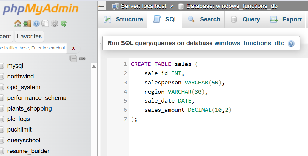
Sample Table
CREATE TABLE sales (
    sale_id INT,
    salesperson VARCHAR(50),
    region VARCHAR(30),
    sale_date DATE,
    sales_amount DECIMAL(10,2)
);
Now let’s insert some sample records.
INSERT INTO sales
(sale_id, salesperson, region, sale_date, sales_amount)
VALUES
(1, 'Amit', 'North', '2026-01-05', 12000),
(2, 'Rahul', 'North', '2026-01-10', 15000),
(3, 'Priya', 'North', '2026-01-15', 18000),
(4, 'Neha', 'North', '2026-01-20', 11000),
(5, 'Amit', 'South', '2026-01-05', 22000),
(6, 'Rahul', 'South', '2026-01-10', 17000),
(7, 'Priya', 'South', '2026-01-15', 25000),
(8, 'Neha', 'South', '2026-01-20', 14000);
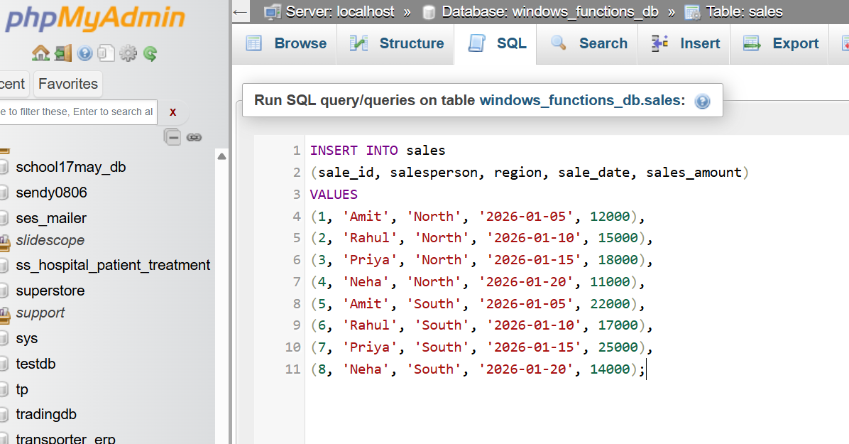
The table looks like this:
| sale_id | salesperson | region | sale_date | sales_amount |
|---|---|---|---|---|
| 1 | Amit | North | 2026-01-05 | 12,000 |
| 2 | Rahul | North | 2026-01-10 | 15,000 |
| 3 | Priya | North | 2026-01-15 | 18,000 |
| 4 | Neha | North | 2026-01-20 | 11,000 |
| 5 | Amit | South | 2026-01-05 | 22,000 |
| 6 | Rahul | South | 2026-01-10 | 17,000 |
| 7 | Priya | South | 2026-01-15 | 25,000 |
| 8 | Neha | South | 2026-01-20 | 14,000 |
Now let’s use this table to understand the three functions.
3. LAG() Function
The LAG() function allows us to access a value from a previous row without using a self-join.
This is particularly useful when we want to answer questions such as:
- How much did sales increase compared with the previous day?
- What was the previous month’s revenue?
- How has a customer’s purchase changed from their previous transaction?
Basic Syntax
LAG(column_name)
OVER (
    ORDER BY column_name
)
You can also specify how many rows backward you want to look.
LAG(column_name, 2)
OVER (
    ORDER BY column_name
)
Here, 2 means that SQL should look two rows back.
LAG Example 1: Compare Current Sale With Previous Sale
Suppose we want to compare each sale with the previous sale.
SQL Command
SELECT
    sale_id,
    sale_date,
    sales_amount,
    LAG(sales_amount) OVER (
        ORDER BY sale_date
    ) AS previous_sale
FROM sales
WHERE region = 'North'
ORDER BY sale_date;
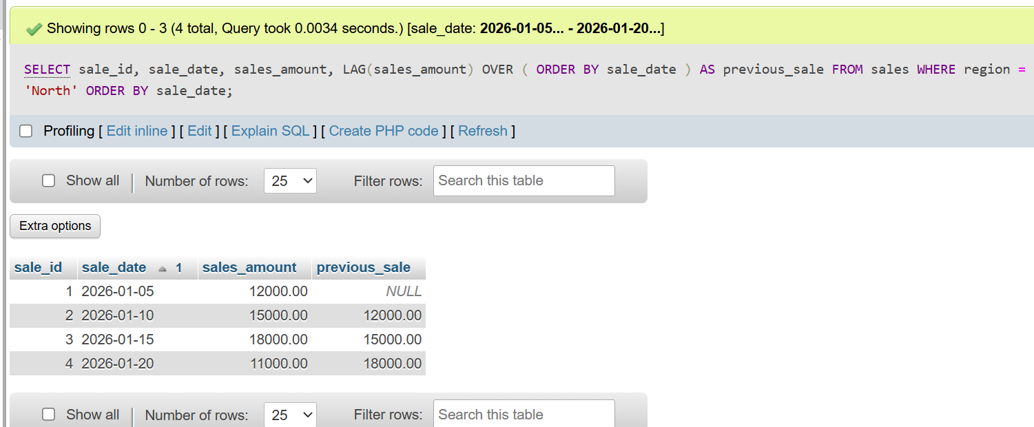
Possible Output
| sale_id | sale_date | sales_amount | previous_sale |
|---|---|---|---|
| 1 | 2026-01-05 | 12,000 | NULL |
| 2 | 2026-01-10 | 15,000 | 12,000 |
| 3 | 2026-01-15 | 18,000 | 15,000 |
| 4 | 2026-01-20 | 11,000 | 18,000 |
The first row contains NULL because there is no previous record.
We can also calculate the difference.
SELECT
    sale_date,
    sales_amount,
    LAG(sales_amount) OVER (
        ORDER BY sale_date
    ) AS previous_sale,
    sales_amount -
    LAG(sales_amount) OVER (
        ORDER BY sale_date
    ) AS sales_difference
FROM sales
WHERE region = 'North'
ORDER BY sale_date;
This allows us to identify whether sales increased or decreased compared with the previous transaction.
LAG Example 2: Compare Sales Separately by Region
LAG() becomes even more useful when combined with PARTITION BY.
Suppose we want to compare each sale with the previous sale within the same region.
SQL Command
SELECT
    region,
    sale_date,
    sales_amount,
    LAG(sales_amount) OVER (
        PARTITION BY region
        ORDER BY sale_date
    ) AS previous_region_sale
FROM sales
ORDER BY region, sale_date;
Possible Output
| region | sale_date | sales_amount | previous_region_sale |
|---|---|---|---|
| North | 2026-01-05 | 12,000 | NULL |
| North | 2026-01-10 | 15,000 | 12,000 |
| North | 2026-01-15 | 18,000 | 15,000 |
| North | 2026-01-20 | 11,000 | 18,000 |
| South | 2026-01-05 | 22,000 | NULL |
| South | 2026-01-10 | 17,000 | 22,000 |
| South | 2026-01-15 | 25,000 | 17,000 |
| South | 2026-01-20 | 14,000 | 25,000 |
Notice that the South region starts again with NULL. This happens because PARTITION BY region creates an independent window for each region.
4. LEAD() Function
While LAG() looks backward, LEAD() looks forward.
It allows us to retrieve a value from a subsequent row.
This is useful when analyzing:
- Future sales
- Next customer transaction
- Next scheduled event
- Next month’s revenue
- Changes between current and future performance
Basic Syntax
LEAD(column_name)
OVER (
    ORDER BY column_name
)
LEAD Example 1: Find the Next Sale
Suppose we want to see the next sale after each transaction.
SQL Command
SELECT
    sale_id,
    sale_date,
    sales_amount,
    LEAD(sales_amount) OVER (
        ORDER BY sale_date
    ) AS next_sale
FROM sales
WHERE region = 'North'
ORDER BY sale_date;
Possible Output
| sale_id | sale_date | sales_amount | next_sale |
|---|---|---|---|
| 1 | 2026-01-05 | 12,000 | 15,000 |
| 2 | 2026-01-10 | 15,000 | 18,000 |
| 3 | 2026-01-15 | 18,000 | 11,000 |
| 4 | 2026-01-20 | 11,000 | NULL |
The final row contains NULL because there is no future record.
We can also calculate the difference between the current and next sale.
SELECT
    sale_date,
    sales_amount,
    LEAD(sales_amount) OVER (
        ORDER BY sale_date
    ) AS next_sale,
    LEAD(sales_amount) OVER (
        ORDER BY sale_date
    ) - sales_amount AS future_difference
FROM sales
WHERE region = 'North'
ORDER BY sale_date;
This can be useful for identifying expected increases or decreases in sequential data.
LEAD Example 2: Find the Next Sale Within Each Region
Now let’s divide our data by region.
SQL Command
SELECT
    region,
    sale_date,
    sales_amount,
    LEAD(sales_amount) OVER (
        PARTITION BY region
        ORDER BY sale_date
    ) AS next_region_sale
FROM sales
ORDER BY region, sale_date;
Possible Output
| region | sale_date | sales_amount | next_region_sale |
|---|---|---|---|
| North | 2026-01-05 | 12,000 | 15,000 |
| North | 2026-01-10 | 15,000 | 18,000 |
| North | 2026-01-15 | 18,000 | 11,000 |
| North | 2026-01-20 | 11,000 | NULL |
| South | 2026-01-05 | 22,000 | 17,000 |
| South | 2026-01-10 | 17,000 | 25,000 |
| South | 2026-01-15 | 25,000 | 14,000 |
| South | 2026-01-20 | 14,000 | NULL |
The important concept here is that LEAD() does not simply look at the next physical row in the table. It looks at the next row according to the ordering defined inside the window.
5. NTILE() Function
The NTILE() function divides an ordered result set into a specified number of approximately equal groups.
For example:
NTILE(4)
divides the rows into four groups.
This is extremely useful in business analytics because we can create:
- Top 25% customers
- Bottom 25% customers
- Sales performance quartiles
- Customer segments
- Employee performance groups
- Revenue tiers
Basic Syntax
NTILE(number_of_groups)
OVER (
    ORDER BY column_name
)
NTILE Example 1: Divide Sales Into Four Quartiles
Suppose we want to divide all sales into four groups based on sales amount.
SQL Command
SELECT
    sale_id,
    salesperson,
    sales_amount,
    NTILE(4) OVER (
        ORDER BY sales_amount DESC
    ) AS sales_quartile
FROM sales;
Possible Output
| sale_id | salesperson | sales_amount | sales_quartile |
|---|---|---|---|
| 7 | Priya | 25,000 | 1 |
| 5 | Amit | 22,000 | 1 |
| 3 | Priya | 18,000 | 2 |
| 6 | Rahul | 17,000 | 2 |
| 2 | Rahul | 15,000 | 3 |
| 8 | Neha | 14,000 | 3 |
| 1 | Amit | 12,000 | 4 |
| 4 | Neha | 11,000 | 4 |
Here:
- Quartile 1 contains the highest-performing sales.
- Quartile 2 contains the next group.
- Quartile 3 contains the next group.
- Quartile 4 contains the lowest sales.
Because we used DESC, the highest sales are placed into group 1.
If you use ASC, the lowest values will be placed into group 1.
NTILE Example 2: Divide Salespeople Into Performance Groups by Region
We can combine NTILE() with PARTITION BY.
Suppose management wants to classify salespeople separately within each region.
SQL Command
SELECT
    region,
    salesperson,
    sales_amount,
    NTILE(2) OVER (
        PARTITION BY region
        ORDER BY sales_amount DESC
    ) AS performance_group
FROM sales
ORDER BY region, performance_group;
Possible Output
| region | salesperson | sales_amount | performance_group |
|---|---|---|---|
| North | Priya | 18,000 | 1 |
| North | Rahul | 15,000 | 1 |
| North | Amit | 12,000 | 2 |
| North | Neha | 11,000 | 2 |
| South | Priya | 25,000 | 1 |
| South | Amit | 22,000 | 1 |
| South | Rahul | 17,000 | 2 |
| South | Neha | 14,000 | 2 |
Here, NTILE(2) creates two groups within each region.
This could be interpreted as:
- Group 1 → Higher-performing sales
- Group 2 → Lower-performing sales
This type of segmentation is useful when a company wants to compare employees against others working in the same region rather than against the entire organization.
6. LEAD vs LAG vs NTILE
Although all three functions are window functions, they solve different analytical problems.
| Function | Purpose | Direction/Method |
|---|---|---|
LAG() | Access a previous row | Looks backward |
LEAD() | Access a following row | Looks forward |
NTILE() | Divide rows into groups | Creates buckets |
A simple way to remember them is:
LAG = Previous
LEAD = Next
NTILE = Groups
For example, if you are analyzing monthly revenue:
January → February → March → April
LAG() can help you compare February with January.
LEAD() can help you compare February with March.
NTILE() can divide your customers or transactions into performance groups.
7. Why Window Functions Matter in Data Analytics
Window functions are particularly valuable because they allow analysts to perform advanced calculations without losing row-level detail.
Consider a sales dashboard.
A traditional GROUP BY query might return:
Region | Total Sales
North  | 56,000
South  | 78,000
That is useful, but the individual transactions are no longer visible.
With a window function, you can keep every transaction and add analytical information to each row.
For example:
SELECT
    region,
    salesperson,
    sales_amount,
    LAG(sales_amount) OVER (
        PARTITION BY region
        ORDER BY sale_date
    ) AS previous_sale
FROM sales;
Now every transaction remains available while SQL also tells us what happened previously.
This is one of the major reasons window functions are widely used in SQL analytics, business intelligence, reporting, financial analysis, and data science workflows.
8. Common Mistakes to Avoid
1. Forgetting ORDER BY
Functions such as LAG() and LEAD() depend heavily on ordering.
This:
LAG(sales_amount) OVER ()
does not clearly define which record should be considered previous.
Prefer:
LAG(sales_amount) OVER (
    ORDER BY sale_date
)
2. Using the Wrong Partition
If you need a comparison within each region, use:
PARTITION BY region
Otherwise, SQL may compare a North transaction with a South transaction.
3. Misunderstanding NTILE()
NTILE(4) does not necessarily mean each group will contain exactly the same number of records when the total number of rows cannot be evenly divided.
SQL distributes the rows as evenly as possible.
4. Ignoring NULL Values
The first row for LAG() and the final row for LEAD() normally return NULL when there is no corresponding previous or next row.
You can handle this with COALESCE() when appropriate.
For example:
COALESCE(
    LAG(sales_amount) OVER (ORDER BY sale_date),
    0
)
Conclusion
SQL analytical window functions provide a powerful way to analyze sequential and grouped data while preserving individual records.
LAG() is ideal when you need to look backward. It can help compare current sales with previous sales, previous transactions, previous months, or previous performance measurements.
LEAD() works in the opposite direction. It allows you to look forward and identify the next transaction, next period, or future value.
NTILE() solves a different problem. Instead of looking backward or forward, it divides ordered records into approximately equal groups. This makes it useful for creating performance tiers, quartiles, customer segments, and ranking-based classifications.
The real strength of these functions appears when they are combined with PARTITION BY and ORDER BY. PARTITION BY allows us to perform calculations independently for different categories, while ORDER BY establishes the sequence used by the analytical calculation.
As a data analyst, I recommend becoming comfortable with these three functions early in your SQL journey. They appear frequently in real-world analytical queries and are especially useful when working with reporting databases, dashboards, financial data, sales data, customer behavior, and business intelligence systems.
A simple mental model is enough to remember them:
LAG looks backward. LEAD looks forward. NTILE creates groups.
Once these concepts become familiar, many analytical SQL problems that initially seem complicated become much easier to solve.